The Physical Structure and Evolution of Transition Region Explosive Events Observed with ESIS

Hi everyone, thanks for coming.

My name is Roy Smart and I’m a PhD student at Montana State University

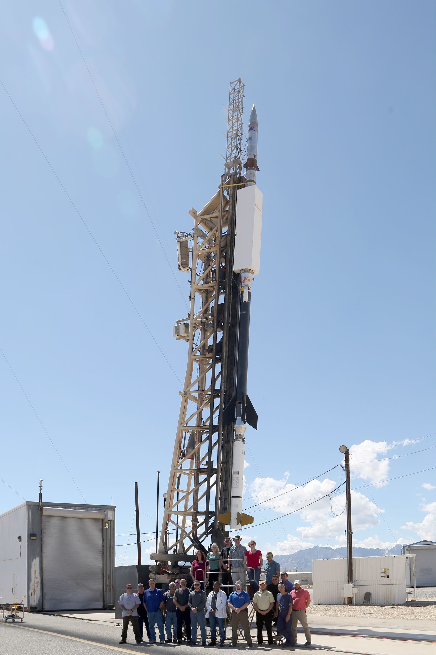
Today I’d like to talk about an event we observed with the EUV snapshot imaging spectrograph, or ESIS, which is a sounding rocket-based instrument we flew in 2019.

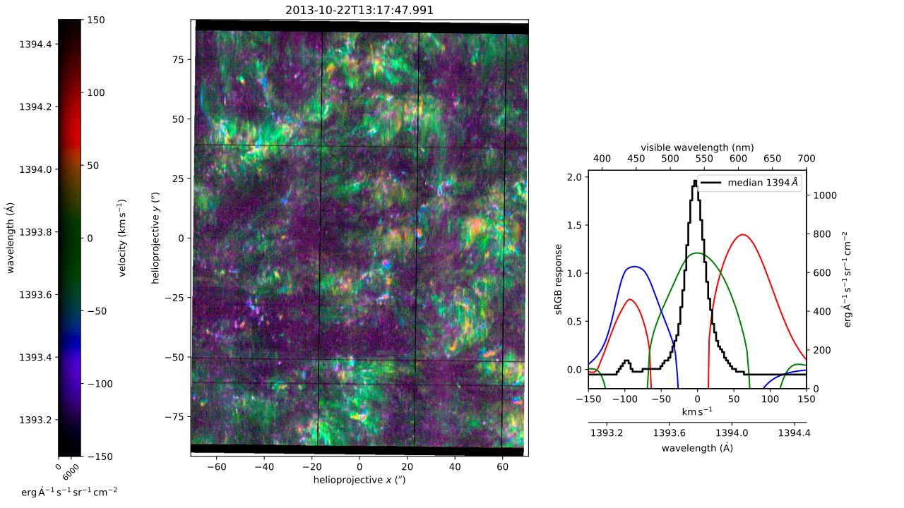
On the left is an example of a deep IRIS raster of the Si IV 1394 Angstrom line in quiet sun conditions near disk center.

This 3D raster is displayed as a 2D false-color image by integrating each line profile against the response of our eyes to the primary colors in our RGB displays.

Colorizing profiles in this way displays a typical profile as pure green, Doppler-shifted profiles as red or blue, and broadened profiles as white or pink.

Looking carefully at this IRIS raster, we can see many small regions of red and blue at arcsecond scales.

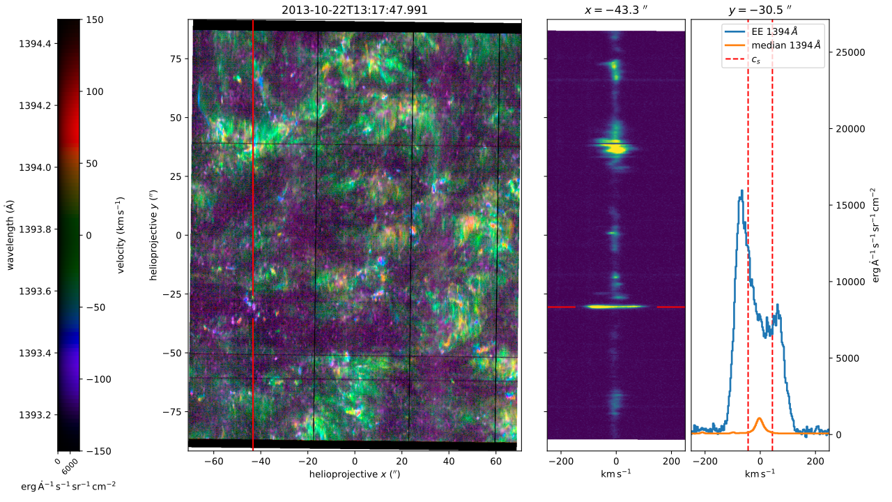
If we look at the line profile of one of these events, we can see that the spectrum of this profile is very broad and bright compared to the median line profile, plotted here in orange, and has supersonic red and blueshifted components.

This is an example of a quiet sun transition region explosive event or TREE, which are small, transient events with significant emission in the wings of TR emission lines.

TREEs are thought to be an observational signature of bidirectional jets formed due to magnetic reconnection, but studying the small-scale spatial dynamics of these events using rastering slit spectrographs, such as IRIS, is limited by the intrinsic tradeoff between FOV and cadence of these instruments.

To get a better understanding of these events, we have developed and flown ESIS, which is an instrument composed of four independent slitless spectrographs, each with a different dispersion direction.

ESIS is designed to primarily observe the O V 630 angstrom line, which is a bright, isolated transition region line formed at about 250,000 K.

On the left is an animation which shows the IRIS raster we considered earlier, shifted and scaled to simulate the brightness and width of the O V line, and then passed through the ESIS forward model.

This demonstrates how the dispersion in each channel spreads the spectrum in a different direction.

Of course, ESIS can’t see these colors directly, what it really sees are these four grayscale images.

The goal of ESIS data analysis is then to invert these four images to recover the corresponding spatial-spectral cube.

Successfully inverting these images allows us to measure the profiles of a few emission lines with high spatial, spectral, and temporal resolution over a wide field of view.

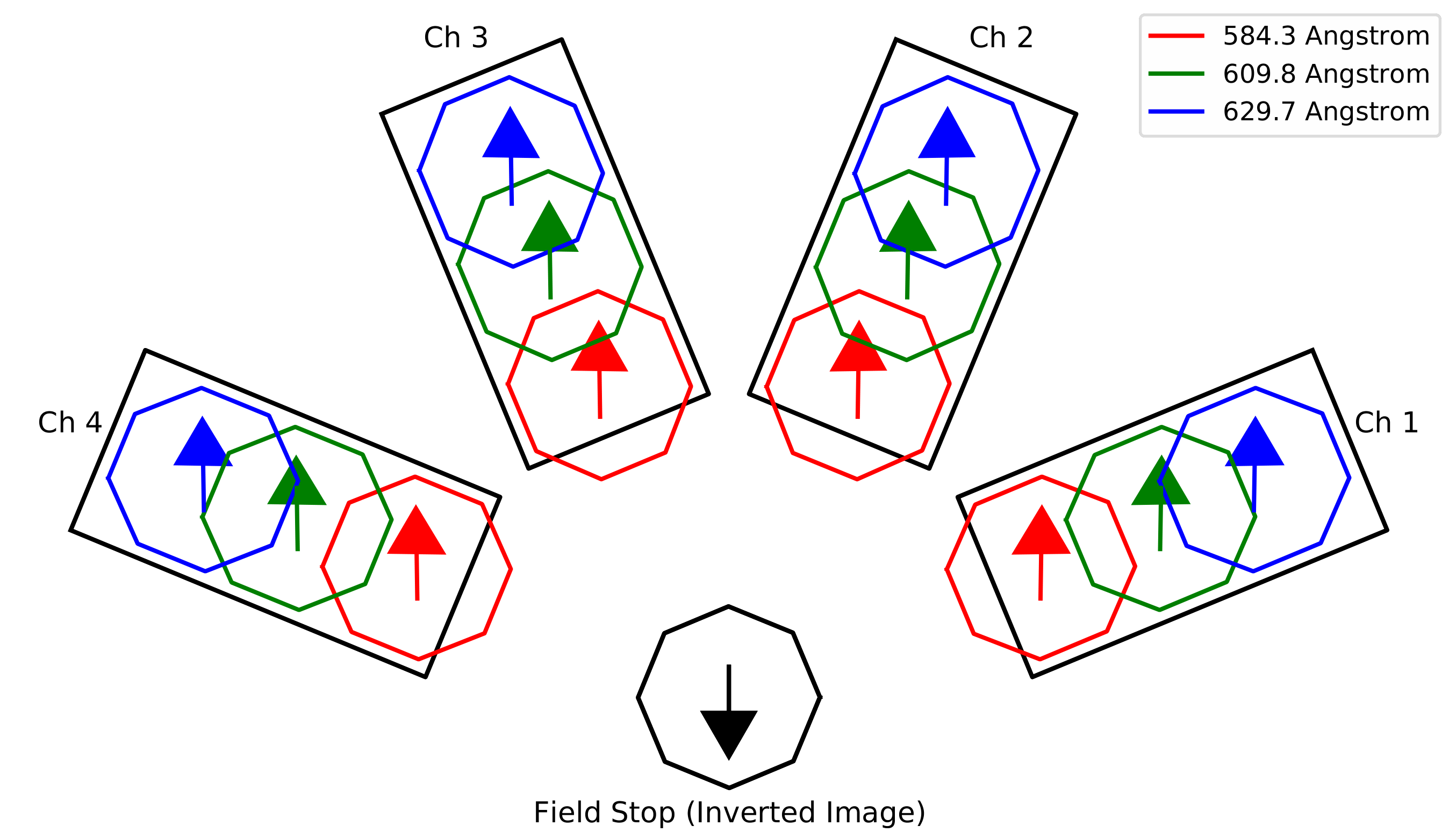
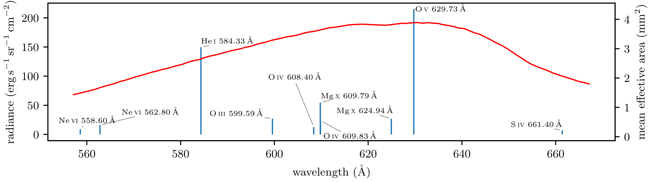
On the top is the spectrum of the ESIS passband which runs from about 560 to 660 angstroms.

Here, we’ve plotted the ten brightest spectral lines in the passband, and of note is the O V 630 A line I mentioned before, as well as two O IV lines at 609 and 608, an O III line at 600, a He I line at 584, and two Mg X lines at 610 and 625 Angstroms.

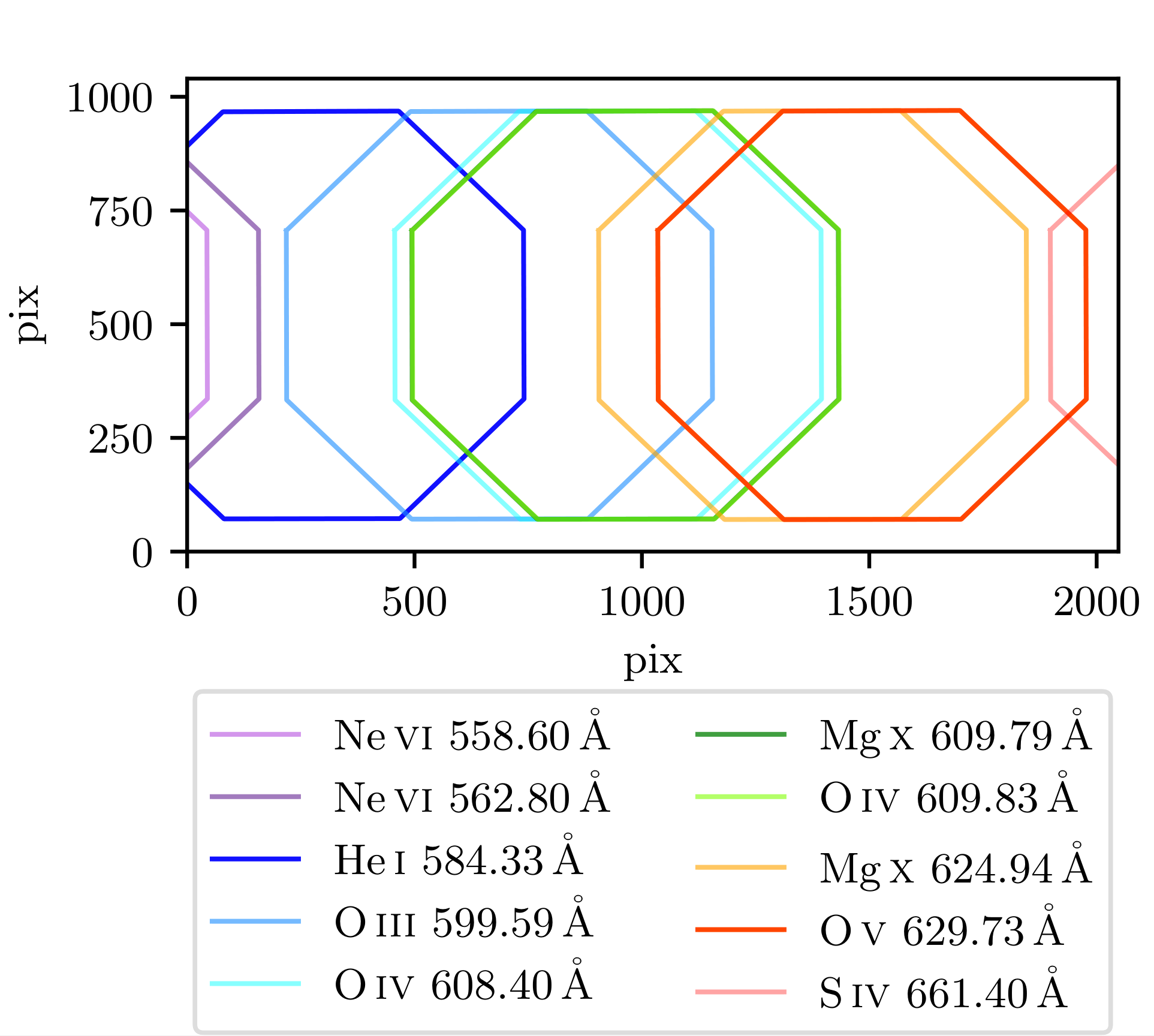
On the bottom left are the same lines as they would appear on the ESIS detector.

ESIS has an octagonal field stop, so each ESIS image is composed of many overlapping octagons from the different emission lines within the passband.

These types of images are often called overlappograms, the only difference with ESIS is that it measures four overlappograms per exposure.

On the right is a schematic showing how each of these overlappograms is oriented around the field stop in 45 degree increments.

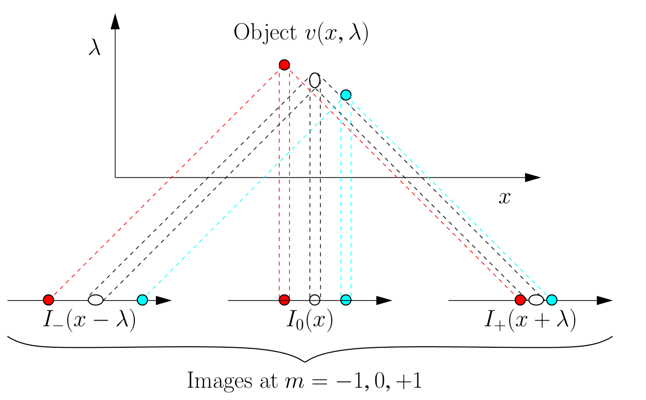
Inverting ESIS observations is equivalent to solving a computed tomography problem.

Computed tomography is commonly used in the medical field to recover the 3D structure of the human body from a series of 2D images, each taken at a different angle.

This is often called a CT scan, and it uses hundreds of images to recover the 3D structure, but ESIS only captures four images, so inverting these observations is ill-posed.

To solve this problem, we employ the multiplicative algebraic reconstruction technique, or MART, which is a classic algorithm used for tomography and is well-suited to the limited number of angles.

On the left is an example of MART being used In a medical context and we can see that the reconstruction is essentially perfect if you have many projections through the volume.

Here is an example of 50 iterations of MART applied to the IRIS TREE we studied in the earlier slides.

From left to right we have: the original scene (degraded to the nominal ESIS resolution), the MART reconstruction, the residual between the two, and the reconstructed line profile in orange.

We can see that this reconstruction is rather noisy since this ends up being a rather dim event for ESIS.

Nonetheless, the qualitative nature of the event is captured, including the supersonic blueshifted component.

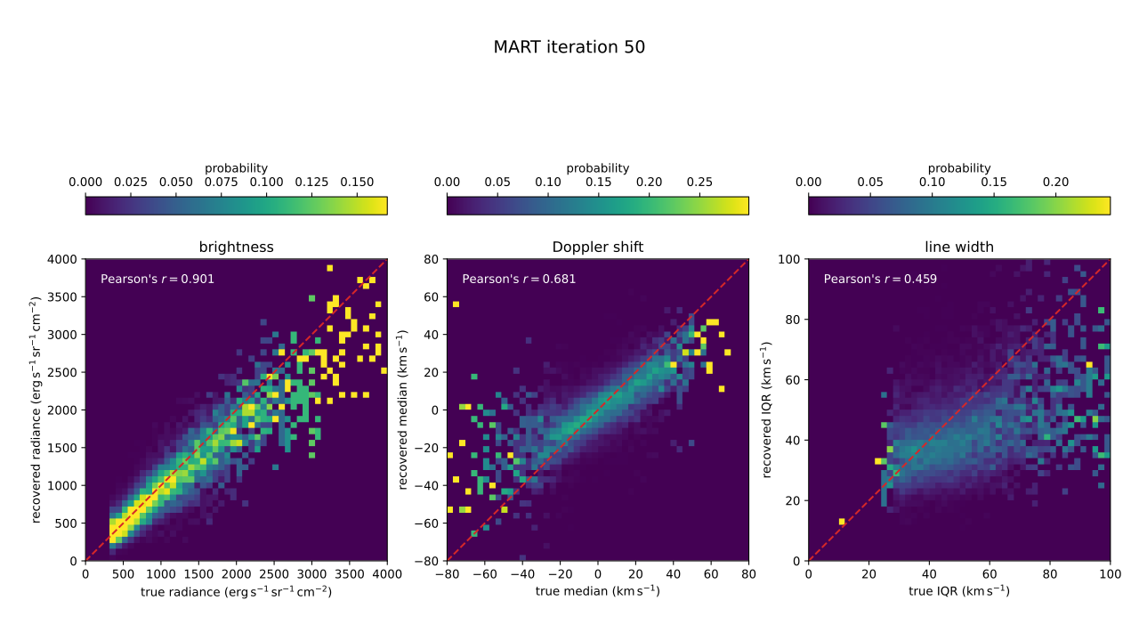
We can also look at the statistical performance this method by analyzing how well the moments of the line profile are reconstructed.

Here is a set of column-normalized 2D histograms comparing the true value of a particular moment against its recovered value for the top 25% brightest pixels in the IRIS raster.

We’ve plotted the first three moments of the line profile: brightness, shift, and width for every iteration of MART so we can inspect the convergence.

If we look at the final iteration, we can see that each successive moment is harder to recover.

We calculated Pearson’s correlation coefficient for each of these moments and found that it was about 0.9 for brightness, 0.68 for shift, and .46 for the width, so MART is much more sensitive to Doppler shifts than it is to widths.

Having hopefully convinced you that MART is a useful algorithm for inverting ESIS observations, we can apply it to real data.

Here are the four ESIS Level-1 image sequences that were input into the MART algorithm.

In total there are 30 frames each with an exposure time of 10 seconds and there’s about 5 minutes of data in total.

We inverted line profiles for the five species I identified in the earlier slide: He I 584, O III 600, O IV 608 + 610, O V 630, and Mg X 610 + 625.

Here is the integrated line intensity for each of these species, and the corresponding AIA 304 images in the bottom right.

We can see that the He I 584, the O III 600, and the O V 630 lines all have similar morphology, with a clearly visible network.

The O IV and the Mg X line are a blended pair at 610 angstroms, so we can see that these two reconstructions look similar despite being formed at different temperatures, so MART may not be fully separating these two lines.

Since we have a line profile for each species, we can display the results as a false-color image in the same way we did with IRIS.

Here is O V as a false-color image, and if we look closely, we can see the many small regions of red and blue that are associated with explosive events.

ESIS observed quiet sun conditions, so the largest event we observed was a tiny jet-like structure that was labeled event E by Parker et al. (2022) and is shown here in this red box.

Here is a zoomed-in animation of that event using data from both ESIS and SDO.

The top row is the integrated intensity, and the second row is the corresponding Doppler shift for each ion recovered by the ESIS inversion.

The third row is AIA 304, 131, 171, and 193 along with the HMI line-of-sight magnetogram.

We can see that this event occurs in an inverted Y structure and is composed of three phases.

In the first phase, the O V doppler map shows blueshifts of about 60 km/s directly adjacent to strong redshifts near the right footpoint of the inverted Y.

As the event progresses, the blueshifted component migrates to the cusp of the inverted Y, while the red component stays near the footpoint.

In the other ionization stages of oxygen we can see the redshifted footpoint component, but not the blueshifted material at the cusp.

This is likely because these lines are too dim, since the He I 584 window, slightly detects the blueshifted material at the cusp.

Finally, in the third phase, we can see what appears to be a blueshifted blob moving along the right leg of the inverted Y at apparent skyplane speeds of around 100-200 km/s.

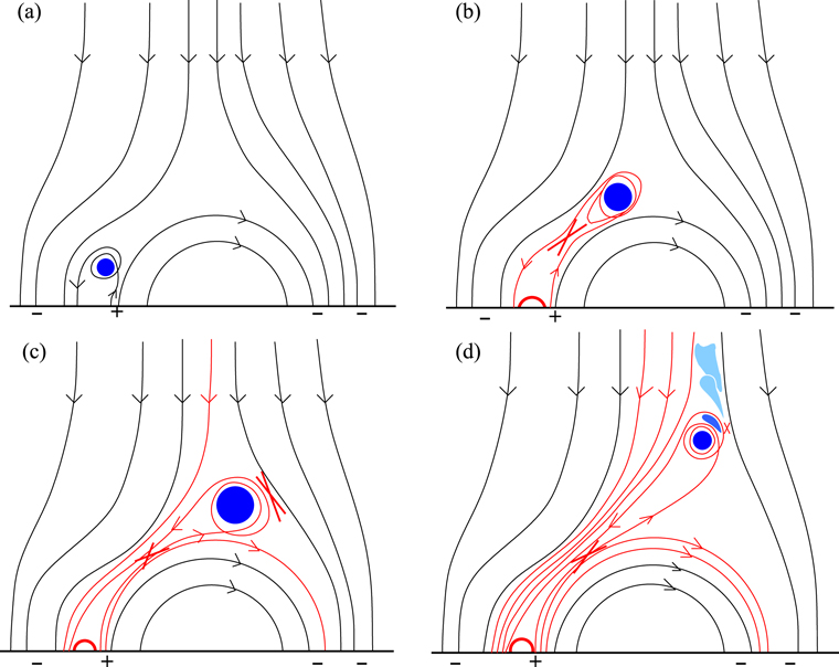
One possible interpretation of this event is that it’s a Sterling et al. style mini filament eruption.

The first phase could be equivalent to panel b of this cartoon from their paper where the rising mini filament undergoes internal reconnection and the two jets are nearly adjacent.

When the blue component of the event moves towards the cusp of the inverted Y in phase 2, this could be a situation like panel c where the minifilament starts reconnecting with the external field.

Phase 3 isn’t necessarily represented by this picture, but it is reminiscent of a plasmoid ejected by the internal reconnection near the footpoint.

Of course, there’s other possible interpretations so we will continue to investigate this event and the other events captured by ESIS.

In conclusion, we found that MART is a useful tool that can invert multiple emission lines within the ESIS passband.

We investigated an event we call Event E, and we found Doppler shifts of at least 60 km/s at the footpoint of an inverted Y structure.

We speculated that Event E might be an example of a Stirling et al. minifilament eruption, and we will continue to investigate this event and other events with better inversion approaches and statistical studies of this dataset.

Thanks!!