Inverting ESIS Observations of the Solar Transition Region
using CNNs
Roy T. Smart, Charles C. Kankelborg, Jacob D. Parker,


Hello everyone and thank you to the organizers for giving me the opportunity to speak today.
My name is Roy Smart and I’m a PhD student here at Montana State University and today, I’d like to talk to you about the EUV Snapshot Imaging Spectrograph, or ESIS, a sounding-rocket-based instrument developed by Montana State University and Marshall Space Flight Center.
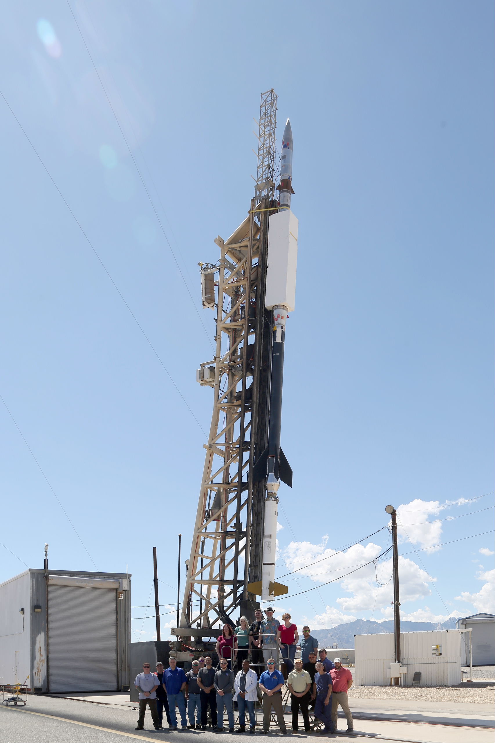
Of course, no sounding rocket talk is complete without a picture of a rocket, so here is a small portion of the ESIS team with the instrument on the pad at White Sands Missile Range in New Mexico before our launch in September 2019.
The EUV Snapshot Imaging Spectrograph (ESIS)
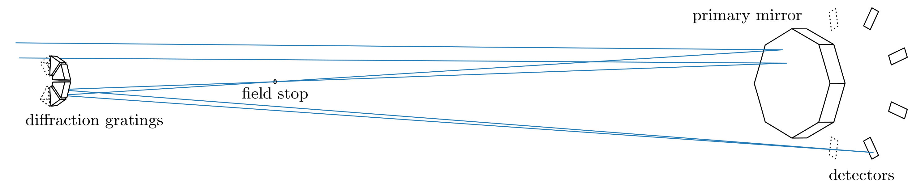
Top: optical layout of the ESIS instrument
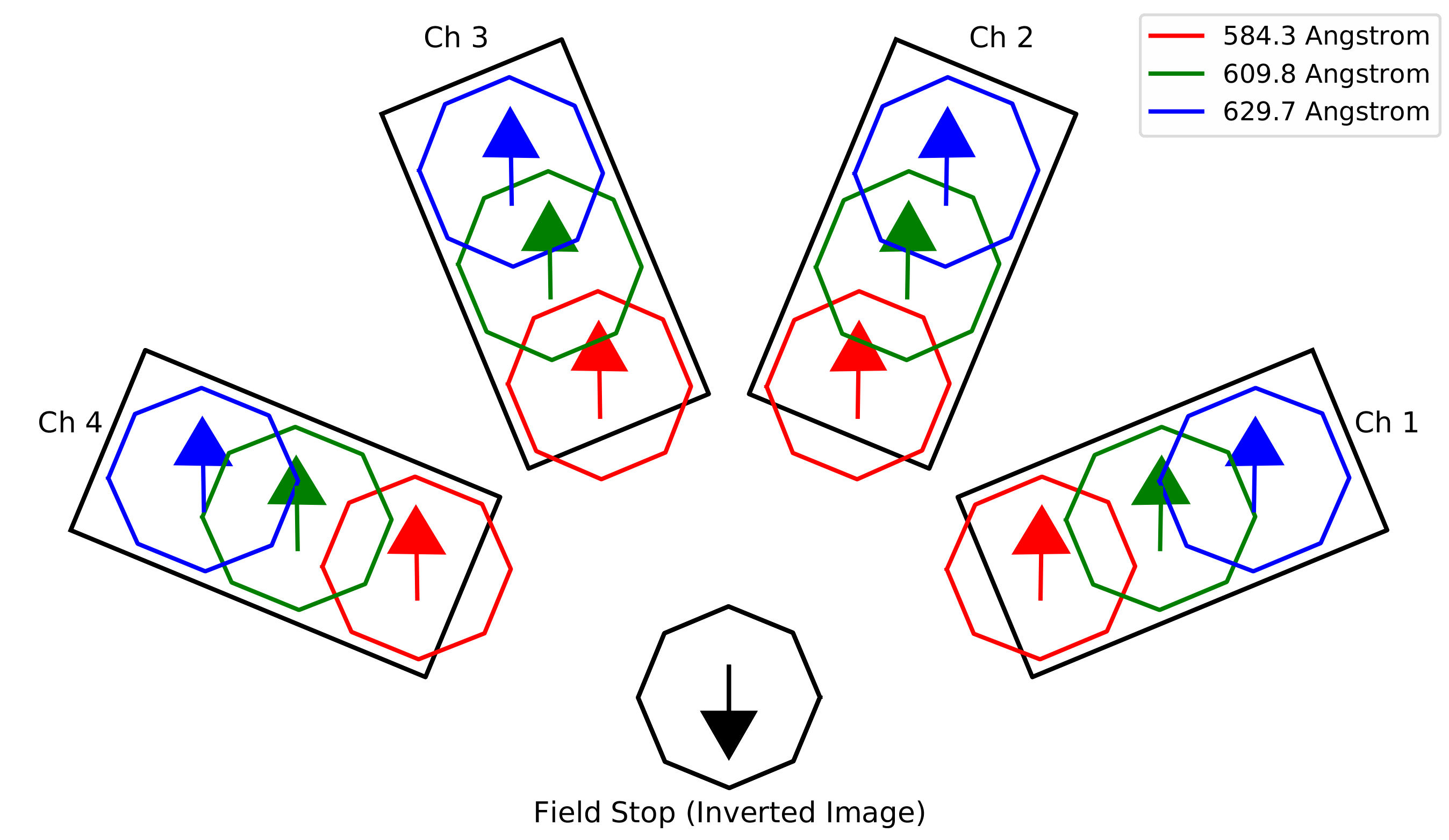
Bottom: ESIS detector schematic
Scene orientation is fixed
Dispersion direction changes
To address this need, ESIS achieves high-cadence imaging spectroscopy in a radical way, it simply deletes the slit from a traditional spectrograph design and allows a wide field of view to be captured by the detector.
Now, that slit was obviously there for a reason, to prevent ambiguity between the spectral axis and the spatial axis perpendicular to the slit.
ESIS resolves this ambiguity by having multiple copies of the spectrograph, each oriented with a different dispersion direction, to provide several independent measurements of a given scene which can be combined with an appropriate inversion algorithm to yield a single spatial-spectral cube for each exposure.
To help visualize how the instrument works, I’ve included a simple schematic of the instrument on the top of this slide.
Light enters from the left and is focused by a primary mirror onto an octagonal field stop.
From there, the light is then dispersed and reimaged by four independent, concave diffraction gratings onto four different detectors on the right side of the image.
On the bottom, I’ve plotted a diagram of how the border of the field stop is projected onto the three detectors.
What I want to draw your attention to is that the orientation of the arrow (which represents the scene) is the same for all four detectors, but the dispersion direction is different.
For the rest of this talk, I will usually only show one channel for simplicity, but I want to emphasize that every ESIS image has three other corresponding images from the other channels.
On the bottom, I’ve plotted the passband of ESIS, which runs from about 550 – 660 Angstroms along with the effective area of the instrument plotted in red.
The dominant lines in this spectral range are the O V 630 Angstrom line and the He I 584 Angstrom line.
In this talk I will be focusing on the O V 630 spectral line since it is the simplest to analyze.
He I 584 A
O V 630 A
Mg X 610 A
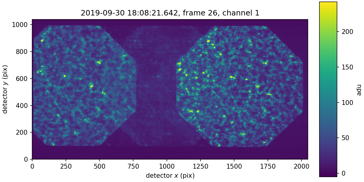
Here is an example of a real ESIS image taken at the apogee of our 2019 flight.
ESIS observes three main spectral lines: He I 584 Anstroms
The O V line is on the right side of the image, the He I is on the left side, and there’s a Mg X line faintly visible between the two.
If you look closely, you may be able to see other spectral lines, but we usually only consider these three lines.
ESIS Inversions
Analogue of a tomographic inversion problem
Spatial/spectral ambiguity
Limited number of angles
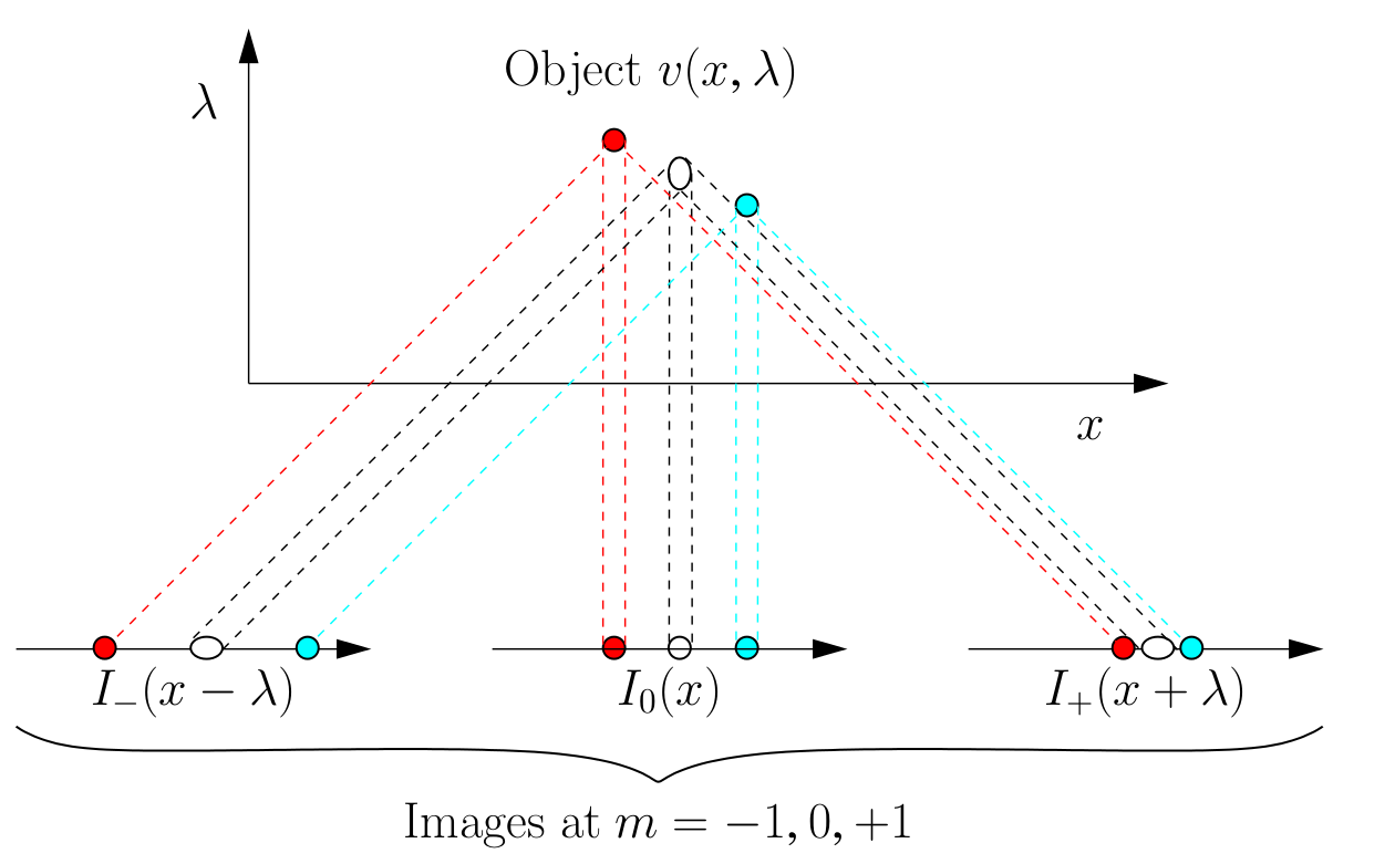
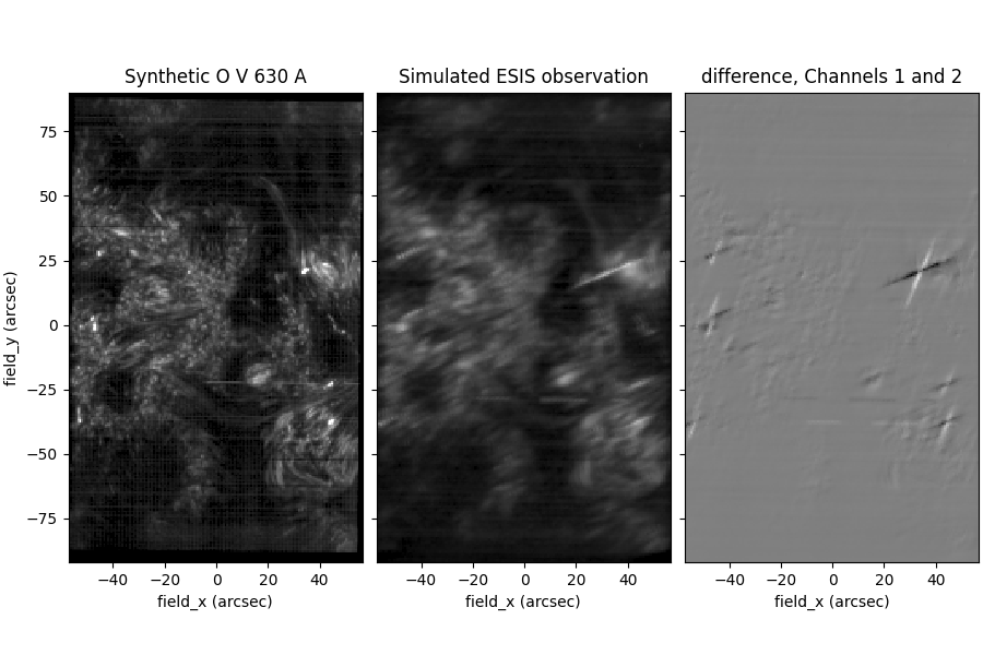
Now, the difference movies are interesting, but they are a qualitative rather than a quantitative analysis.
What we’re really after is a spatial-spectral cube, which is a data product with a spectral line profile for every point in a 2D scene.
Generally, the spatial-spectral cube we desire has on the order of 10-20 points along the spectral axis, but ESIS only has four independent channels, so recovering the spatial-spectral cube from ESIS imagery is an ill-posed inversion problem since the result has about 4x more information than the inputs.
Mathematically speaking, this inversion problem is analogous to a tomographic reconstruction problem, like what is done in the medical field when they take X-ray images from many different angles around your body to get a 3D view of your internal organs
The difference with instruments like ESIS is that instead of trying to reconstruct an object in three spatial dimensions, we’re trying to reconstruct an object with two spatial dimensions and one spectral dimension.
One of the simplest tomographic reconstruction algorithms is known as the multiplicative algebraic reconstruction technique or MART.
This algorithm projects all the images back through the three-dimensional volume and then multiplies them together to reconstruct the 3D volume, and on the left is an example of that technique from a CT scan.
Convolutional Neural Network inversion technique
Training/validation dataset
IRIS Si IV 1394 A 320-step dense rasters
Scaled to average O V linewidth
Rebinned to ESIS resolution
64 training / 17 validation examples
Network Architecture
Fully-convolutional network
2 convolutional + 2 deconvolutional layers
11x11x11 kernel size
32 filters per layer
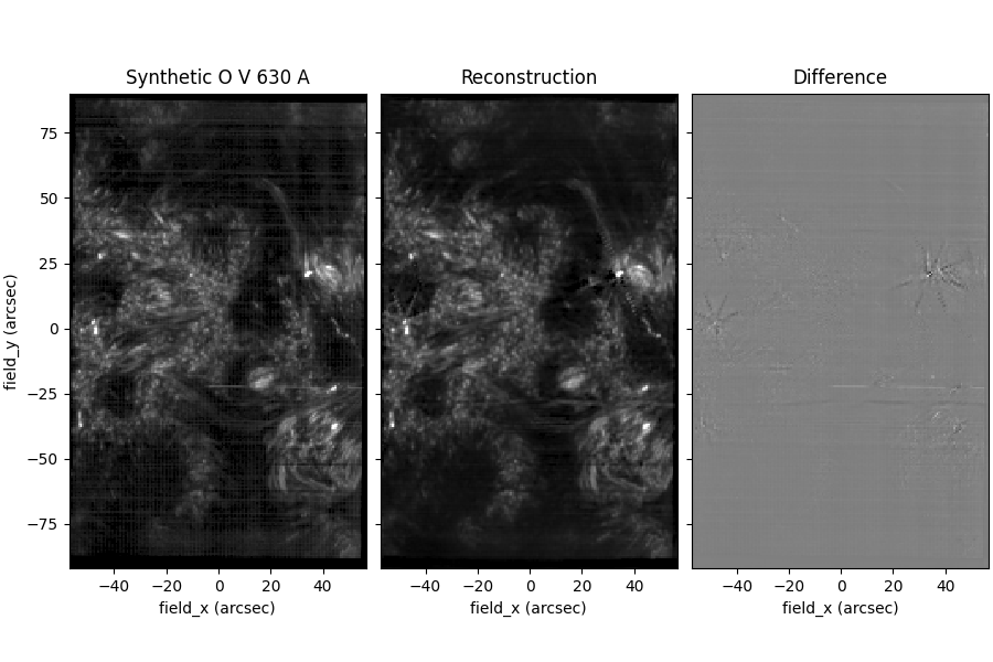
A very trendy technique right now which can represent this statistical model is a convolutional neural network, or CNN.
CNNs are often used for image classification tasks, but they can be also used for regression problems like the ESIS inversion problem where we’re trying to fit the relationship between the observed images and the associated spatial-spectral cube.
In broad terms, a CNN used in this way is a type of universal filter with many free parameters that are iteratively adjusted during training to best fit the data.
In broad terms, we simply provide ESIS imagery as an input to the network, and we train it to reconstruct the associated spatial-spectral cube by giving feedback in terms of the Euclidean distance between the network output and the target cube.
The network has
In broad terms, a convolutional neural network is an arbitrary nonlinear filter, which can be trained to invert ESIS observations by presenting it with many examples of ESIS imagery along with the associated spatial-spectral cube to provide feedback to the network.
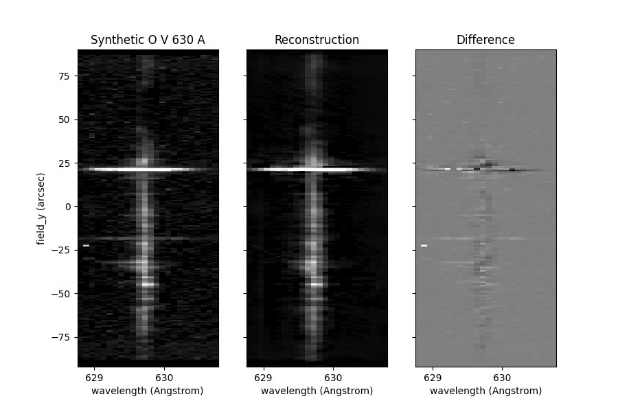
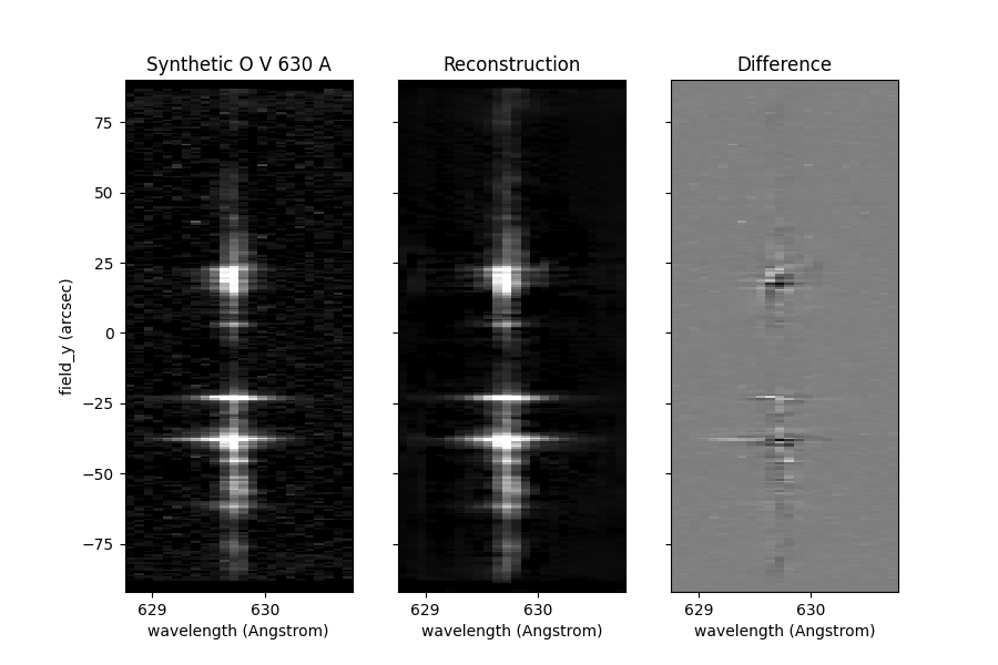
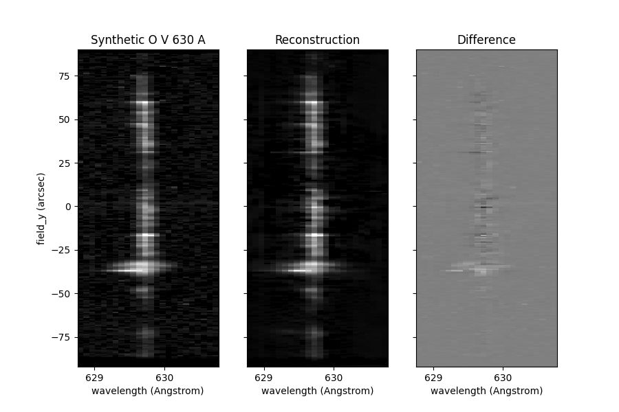
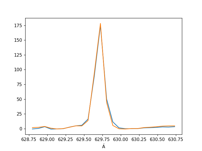
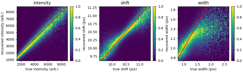
Top: true-vs-reconstructed histogram for first three moments of the line profile using the 25% brightest pixels in validation dataset.
Right: Average validation spectrum (blue), average reconstructed spectrum (orange)